Power and Sample Size Estimation for Microbiome Analysis
Michael Agronah and Benjamin Bolker
2026-06-12
Source:vignettes/stub.rmd
stub.rmdPackage Description and Functionalities
power.nb is a package developed for estimating
statistical power and required sample size in differential abundance
microbiome studies using negative binomial models. The package includes
tools for simulation-based power analysis and sample size estimation
using generalized additive models (GAMs), and visualization utilities
for exploring the relationship between power, effect size, abundance,
and sample size.
power.nb presents two novel microbiome data simulations
frameworks: the Mixture of Gaussians (MixGaussSim) and the Reduced Rank
(RRSim) simulation approaches. MixGaussSim models the distribution of
mean abundance of taxa and the distribution of fold change (as a
function of mean abundance of taxa) by finite Mixture of Gaussian
distributions. Microbiome count data is then simulated from a negative
binomial distribution. Detailed description of the MixGaussSim method is
presented in the paper “Investigating
statistical power of differential abundance studies” (Agronah and Bolker 2025).
RRSim (this simulation method is still under development and some
functions in RRSim are yet to tested), on the other hand models the mean
abundance of all taxa jointly with a mixed-effects model while
accounting for correlations among taxa within subjects and zero
inflation in microbiome data. Given the high dimensionality of
microbiome data (usually having hundreds or thousands of taxa),
modelling correlations between taxa requires estimating thousands or
even millions of parameters for the correlation matrix. RRSim uses the
reduced rank functionality implemented in the glmmTMB (Magnusson et al. 2017) packages to reduce the
number of parameter estimates required of the variance-correlation
matrix. Details of this method is presented in the thesis “A Novel
Approach for Simulation-Based Power Estimation and Joint Modeling of
Microbiome Counts” (Agronah 2025)
Installation
Install the package from GitHub using devtools:
install.packages("devtools")
devtools::install_github("magronah/power.nb")
Simulating microbiome data
Since the goal of differential abundance studies is to identify taxa that differ significantly between groups, statistical power must be estimated at the level of individual taxa. Because of the complexity of microbiome data, analytical approaches based on theoretical distributions of test statistics (e.g., non-central t or chi-squared distributions) are not feasible (Arnold et al. 2011). Therefore, power estimation typically relies on simulation-based methods that can mimic the characteristics of real microbiome data.
Statistical power for a given taxon depends on both its mean abundance and effect size (defined in this package as fold changes) (Agronah and Bolker 2025). Thus, estimating the distributions of mean abundance and fold change of taxa explicitly will offer great benefit for estimation of statistical power for individual taxon. We use the MixGaussSim simulation approach to simulate microbiome data for power calculation due to its flexibility in modelling the distributions of taxa mean abundances and effect sizes explicitly as as well as their relationship.
Two ways to obtain parameters for data simulation using MixGaussSim
There are one of two ways to obtain the parameters of the MixGaussSim method for data simulation. Users can:
1. pre-specify a set of parameters: To help users decide on plausible parameter values, we have run MixGaussSim on some of the microbiome datasets used in the paper “Microbiome differential abundance methods produce different results across 38 datasets” (Nearing et al. 2022) and presented the parameter estimates obtained from each of these datasets (see Appendix for the parameter estimates from these datasets ).
2. estimate parameters from an existing dataset: Secondly, users can also obtain estimates directly from fitting the model implemented in MixGaussSim to existing datasets. The following steps outlines the process for estimating parameters from an existing dataset.
Dataset
We use a subset of the Obesity dataset, one of the datasets analyzed in (Nearing et al. 2022). The full dataset contains 52 samples and 1203 taxa.
##Load libraries
library(tidyverse)
library(dplyr)
library(power.nb)
library(patchwork)
library(rlist)
library(latex2exp)

data_path =  system.file("pkgdata", package = "power.nb")
##Read count data and metadata
data <- read.table(
  file.path(data_path, "ob_ross_ASVs_table.tsv"),
  header = TRUE, sep = "\t",
  check.names = FALSE, comment.char = "",
  row.names = 1
)

metadata <- read.table(
  file.path(data_path, "ob_ross_metadata.tsv"),
  header = TRUE, sep = "\t",
  check.names = FALSE, comment.char = ""
)

metadata <- metadata %>%
  setNames(c("SampleID", "Groups"))

dim(data); dim(metadata)
## [1] 1203 52## [1] 52 2## BD0017v13 BD0027v13 BD0022v13 BD0040v13 BD0044v13 BD0057v13 BD0115v13
## denovo619 0 0 0 0 0 0 0
## denovo618 0 0 0 0 0 0 0
## BD0190v13 BD0072v13 BD0112v13 BD0246v13 BD0247v13 BD0266v13 BD0235v13
## denovo619 8 0 0 0 0 0 0
## denovo618 0 0 0 0 0 0 0
## BD0295v13 BD0255v13 BD0300v13 BD0331v13 BD0321v13 BD0351v13 BD0409v13
## denovo619 1 0 0 0 0 0 8
## denovo618 0 0 0 0 0 0 0
## BD0410v13 BD0375v13 BD0414v13 BD0422v13 BD0464v13 BD0571v13 BD0578v13
## denovo619 0 0 0 0 0 0 0
## denovo618 0 0 0 0 0 0 1
## BD0587v13 BD0592v13 BD0594v13 BD0610v13 BD0611v13 BD0613v13 BD0636v13
## denovo619 0 0 0 1 0 0 0
## denovo618 2 0 0 0 0 18 0
## BD0616v13 BD0653v13 BD0643v13 BD0654v13 BD0673v13 BD0735v13 BD0760v13
## denovo619 0 0 0 1 0 0 0
## denovo618 0 0 0 0 0 0 0
## BD0777v13 BD0758v13 BD0789v13 BD0791v13 BD0821v13 BD0786v13 BD0790v13
## denovo619 0 0 0 0 7 0 0
## denovo618 0 0 0 0 6 0 0
## BD0913v13 BD0954v13 BD0981v13
## denovo619 0 0 0
## denovo618 0 0 0## SampleID Groups
## 1 BD0017v13 OB
## 2 BD0027v13 HPre-filtering low abundant taxa
Low abundant tax exhibit high variability, posing challenges in detecting significant differences between groups (Love et al. 2014). Pre-filtering steps, as is routinely done in differential abundance analysis, is used to filter out these low abundant taxa. We filter out taxa with less that 10 count in less that 5 samples.
filter_data  =  filter_low_count(countdata     =  data,
                                metadata       =  metadata,
                                abund_thresh   =  3,
                                sample_thresh  =  2,
                                sample_colname =  "SampleID",
                                group_colname  =  "Groups")

dim(filter_data)
## [1] 707 52Fold change and Dispersion Estimation
We estimate fold change for each taxon and dispersion parameters
using the negative binomial model implemented in the DESeq2
package (Love et al. 2014). The negative
binomial model is widely used in both microbiome and RNA-seq analyses
and is implemented in the NBZIMM (Yi
2020) and edgeR R packages (Robinson et al. 2010). The model implemented in
the DESeq2 package is described as follows:
Let
represent the observed count for the
taxon in the
sample. The model assumes that
where the mean is defined as
,
and
is the normalization factor for sample
.
The expected abundance prior to normalization,
,
is modeled as
with
denoting the covariates and
the associated coefficients. The dispersion parameter is assumed
constant across samples for each taxon, such that
.
This formulation links the variance and mean through
Estimation of the regression coefficients
and dispersion parameters
was carried out using the empirical Bayes shrinkage procedures
implemented in the DESeq2 package Anders and Huber (2010).
unique(metadata$Groups)## [1] "OB" "H"
foldchange_est <- deseqfun(countdata      =   filter_data,
                           metadata       =   metadata,
                           alpha_level    =   0.1,
                           ref_name       =  "H",
                           group_colname  =  "Groups",
                           sample_colname =  "SampleID")

logfoldchange =  foldchange_est$deseq_estimate$log2FoldChange

head(logfoldchange)
## [1] 0.3472147294 -0.8840585417 0.2167456449 -0.5366652659 0.0008622315
## [6] -0.8221867027Modeling the distribution of log mean counts
We modelled the log mean abundance (defined as the logarithm of the arithmetic mean abundance across both control and treatment groups) as a finite mixture of Gaussian distributions. To determine the optimal number of mixture components, denoted by , we employed a parametric bootstrap approach to sequentially compare models with and components.
Let the observed data be denoted by , where each represents the log mean abundance for the taxon. The mixture model with components is given by
where are the mixing proportions satisfying , and denotes the normal density with mean and variance .
To test whether adding an additional component improves model fit, we formulated the hypotheses as:
{=latex}’
The test statistic is the likelihood ratio statistic:
’ where and are the maximized log-likelihoods under the - and -component models, respectively. {=latex}’
To approximate the null distribution of , we performed a parametric bootstrap using bootstrap samples generated under . For each bootstrap replicate , data were simulated from the fitted -component model, and both the null and alternative models were re-fitted to obtain . The empirical -value is computed as
where is the observed likelihood ratio statistic.
If , the null hypothesis is rejected in favor of the -component model. Testing proceeds sequentially for until the -value exceeds the significance threshold, at which point the -component model from the last accepted test is selected as the optimal mixture size (Benaglia et al. 2010).
### function to mute printing out messages about
### update on the number of iterations

quiet <- function(expr) {
  out <- suppressWarnings(suppressMessages(
    capture.output(res <- eval.parent(substitute(expr)))
  ))
  res}

### Path to other files used in this vignette
extdata_path =  system.file("extdata", package = "power.nb")
 logmean    =  log(rowMeans(filter_data))
 logmeanFit <- readRDS(file.path(extdata_path, "logmeanFit.rds"))

## The code below was used to generate the precomputed
## `logmeanFit.rds` object. The saved result is loaded
## throughout this vignette to reduce vignette build times.

# logmeanFit =   quiet(logmean_fit(logmean, sig = 0.05,
#                                  max.comp = 4, max.boot = 100))
Modelling the distribution of log fold change estimates
We also modelled log fold change of taxa as a finite mixture of Gaussian distributions. Fold change is typically related to mean abundance (Love et al. 2014); therefore, we expressed the mean and standard deviation parameters of the individual Gaussian components as functions of log mean abundance. Detailed description of the model fitted to log fold changes is presented in the paper “Investigating statistical power of differential abundance studies” (Agronah and Bolker 2025).
## $par
##  logitprob_1     mu_int_1     mu_int_2   mu_slope_1   mu_slope_2   logsd_.1_1
##  1.688126642 -1.054068569  0.115132772 -0.611302399  0.007166436 -0.554719649
##   logsd_.1_2   logsd_.L_1   logsd_.L_2
## -0.512670667  0.415862601  0.233292472
##
## $np
## [1] 2
##
## $sd_ord
## [1] 1
##
## $aic
## [1] 1609.076
## The code below was used to generate the precomputed
## `logfoldchangeFit.rds` object. The saved result is loaded
## throughout this vignette to reduce vignette build times.

# logfoldchangeFit <- quiet(logfoldchange_fit(logmean,
#                                             logfoldchange,
#                                             ncore = 1,
#                                             max_sd_ord = 2,
#                                             max_np = 5,
#                                             minval = -5,
#                                             maxval = 5,
#                                             itermax = 100,
#                                             NP = 800,
#                                             seed = 100))
Modelling the dispersion estimates
Because dispersion tends to depend on mean count abundance with rarer
taxa showing greater variability we modeled the dispersion as a
nonlinear function of the mean, following the approach implemented in
DESeq2. The nonlinear function is defined by
where and denote the scaled dispersion and mean abundance respectively. The term represents the asymptotic dispersion level for high abundance taxa, and captures additional dispersion variability. This procedure enables estimation of dispersion values corresponding to given mean counts, facilitating their use in downstream simulations and power analyses.
dispersion    =  foldchange_est$dispersion
dispersionFit =  dispersion_fit(dispersion, logmean)
dispersionFit$param
## asymptDisp extraPois
## 1 15.43238 6.246524Simulate count microbiome data
To simulate microbiome data, we first simulate log mean counts and corresponding log fold changes. The simulated log mean counts represent overall log mean counts (i.e., log of the arithmetic mean of the counts in all of treatment and control groups). We then use the simulated log mean count to estimate corresponding dispersion values for each sample through the fitted nonlinear function described in the equation here (see section on Modelling the Distribution of Log Fold Changes). Using the simulated log mean counts and fold changes, we now compute the group specific mean counts (i.e., mean counts of taxa for control group and mean count of taxa for treatment group). We then simulate microbiome count data from the negative binomial distribution using the group specific mean counts and the estimated dispersion values.
Simulate log mean count and log fold change
### Simulated log mean count and log foldchange from the fitted
### log mean count and log foldchange models

logmean_param       =  logmeanFit$param
logfoldchange_param =  logfoldchangeFit

notu  = dim(filter_data)[1]
notu
## [1] 707
logmean_sim  =  logmean_sim_fun(logmean_param, notu)

logfoldchange_sim  =  logfoldchange_sim_fun(logmean_sim = logmean_sim,
                                            logfoldchange_param =
                                            logfoldchange_param,
                                            max_lfc  = 15,
                                            max_iter = 30000)

head(logfoldchange_sim)
## [1] 0.1310574 -0.3036162 -0.2573167 0.2145373 0.1906037 1.1280157Simulate counts from the negative binomial distribution
Estimating the dispersion values is done internally within the
countdata_sim_fun function.
nsim = 4
ntreat = sum(metadata$Groups == "OB")
ncont  = sum(metadata$Groups == "H")
dispersion_param  =  dispersionFit$param

countdata_sims = countdata_sim_fun(logmean_param,
                                   logfoldchange_param,
                                   dispersion_param,
                                   nsamp_per_group = NULL,
                                   ncont = ncont,
                                   ntreat = ntreat,
                                   notu,
                                   nsim = nsim,
                                   disp_scale = 0.7,
                                   max_lfc = 15,
                                   maxlfc_iter = 1000,
                                   seed = 121)
## mixtools package, version 2.0.0.1, Released 2022-12-04
## This package is based upon work supported by the National Science Foundation under Grant No. SES-0518772 and the Chan Zuckerberg Initiative: Essential Open Source Software for Science (Grant No. 2020-255193).
dim(countdata_sims$treat_countdata_list$sim_1)## [1] 707 31
dim(countdata_sims$control_countdata_list$sim_1)## [1] 707 21
dim(countdata_sims$countdata_list$sim_1)## [1] 707 52
dim(countdata_sims$metadata_list$sim_1)## [1] 52 2Comparing the distributions between simulated count d of mean count and fold change from simulation with actual data
We compare the following comparisons between our simulation and the actual dataset
we come distribution of variances of counts of taxa and
the means of taxa from out simulation with those of the actual dataset
compare_dataset <- function(countdata_sim_list,countdata_obs,method = c("var", "mean")){

  # Check if method is either "var" or "mean"
  if (!(method %in% c("var", "mean"))) {
    stop("Invalid method. Please choose either 'var' or 'mean'.")
  }

  # Calculate variance or mean based on the chosen method
  if (method == "var") {
    calc_func <- stats::var
    xlab_text <- "$\\log$(variance of taxa)"
  } else {
    calc_func <- mean
    xlab_text <- "$\\log$(mean of taxa)"
  }

  # Create a list combining simulation data and observed data
  dlist <- list.append(countdata_sim_list, obs_filt = countdata_obs)

  # Calculate variance or mean for each dataset in the list
  vars <- dlist |> purrr::map(~ apply(., 1, calc_func)) |>
    purrr::map_dfr(~ tibble(var = .), .id = "type")

  # Separate observed and simulated data
  vars_obs <- vars[vars$type == "obs_filt", ]
  vars_sim <- vars[vars$type != "obs_filt", ]

  # Create ggplot for visualization
  p <- ggplot(vars_sim, aes(x = log(var), colour = type)) +
    geom_density(lwd = 1.5) +
    geom_density(data = vars_obs, aes(x = log(var)),
                 colour = "black", linetype = "dashed", lwd = 1.5) +
    xlab(TeX(xlab_text)) + theme_bw()

  return(p)
}

countdata_sim_list =  countdata_sims$countdata_list[1]
countdata_obs      =  filter_data
p11 = compare_dataset(countdata_sim_list,countdata_obs,method = "mean")
p12 = compare_dataset(countdata_sim_list,countdata_obs,method = "var")

(p11|p12) + plot_layout(guides = "collect")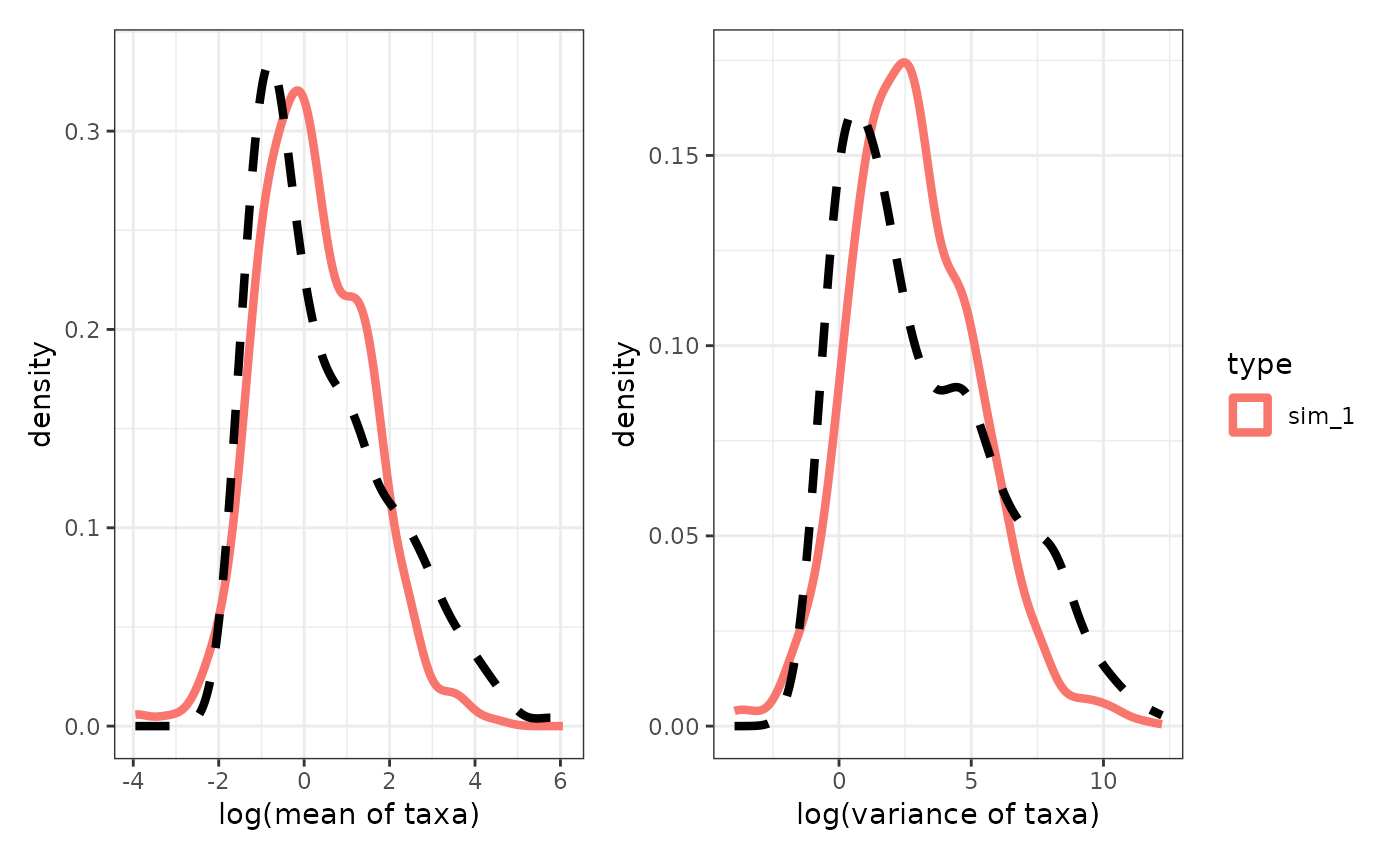
dim(countdata_obs)## [1] 707 52Estimating Statistical Power for Individual Taxa
We estimate statistical power for a given taxon as the probability of rejecting the null hypothesis that the mean abundance in the control and treatment groups are the same for that given taxon. To estimate statistical power for various combinations of log mean abundance and log fold change, we fitted a shape-constrained generalized additive model (GAM) (Pya and Wood 2015). The event that a given taxon is significantly different between groups is treated as a Bernoulli trial.
Define the logistic function as .
The model predicting statistical power as a function of log fold change and log mean abundance is given by:
where:
- is a binary value (1 if the p-value was below the critical threshold, and 0 otherwise);
- is the estimated statistical power for taxon ;
- is the intercept;
- The predictors and represent log mean abundance and log fold change, respectively;
- is a two-dimensional smoothing surface, generated using a tensor product smooth of log mean abundance and log fold change.
Power and fold change are positively correlated. Additionally, effect sizes of highly abundant taxa are more likely to be detected—hence having higher power—than those of rare taxa. To account for these relationships, the function was constrained to be a monotonically increasing function of both log mean abundance and log fold change.
We used the DESeq2 package to compute p-values for each
taxon, applying the Benjamini and Hochberg method for false discovery
rate (FDR) correction. We used the default critical p-value threshold of
0.1 in the DESeq2 package.
The follow steps outlines the power estimation procedure:
Estimate p-values associated with simulated fold changes
To train the GAM on a sufficiently large sample size, we generate
multiple microbiome count datasets following the procedure described in
the section Simulate count
microbiome data. We then estimate p-values associated with the
simulated fold changes using the DESeq2 package.
countdata_list  =   countdata_sims$countdata_list
metadata_list   =   countdata_sims$metadata_list
desq_est   =   quiet(deseq_fun_est(metadata_list =  metadata_list,
                            countdata_list =  countdata_list,
                            alpha_level    =  0.1,
                            group_colname  = "Groups",
                            sample_colname = "Samples",
                            num_cores      =  1,
                            ref_name       = "control"))

deseq_est_list     =    lapply(desq_est, function(x){x$deseq_estimate})
names(desq_est$sim_1)
## [1] "logfoldchange" "dispersion" "deseq_estimate" "normalised_count"
## [5] "deseq_object" "metadata" "countdata"Fitting the Generalized Additive Model (GAM)
We now fit the GAM for predicting statistical power for individual taxon.
true_lmean_list       =    countdata_sims$logmean_list
true_lfoldchange_list =    countdata_sims$logfoldchange_list

gamFit <- gam_fit(deseq_est_list,
                  true_lfoldchange_list,
                  true_lmean_list,
                  grid_len = 50,
                  alpha_level=0.1)

range(true_lfoldchange_list)
## [1] -8.952604 7.643726
range(true_lmean_list)## [1] -2.383209 6.458936Contour plot showing power for various combinations of mean abundance and fold change
cont_breaks     =  seq(0,1,0.1)
combined_data   =  gamFit$combined_data
power_estimate  =  gamFit$power_estimate

contour_plot <- contour_plot_fun(combined_data,
                                 power_estimate,
                                 cont_breaks)
contour_plot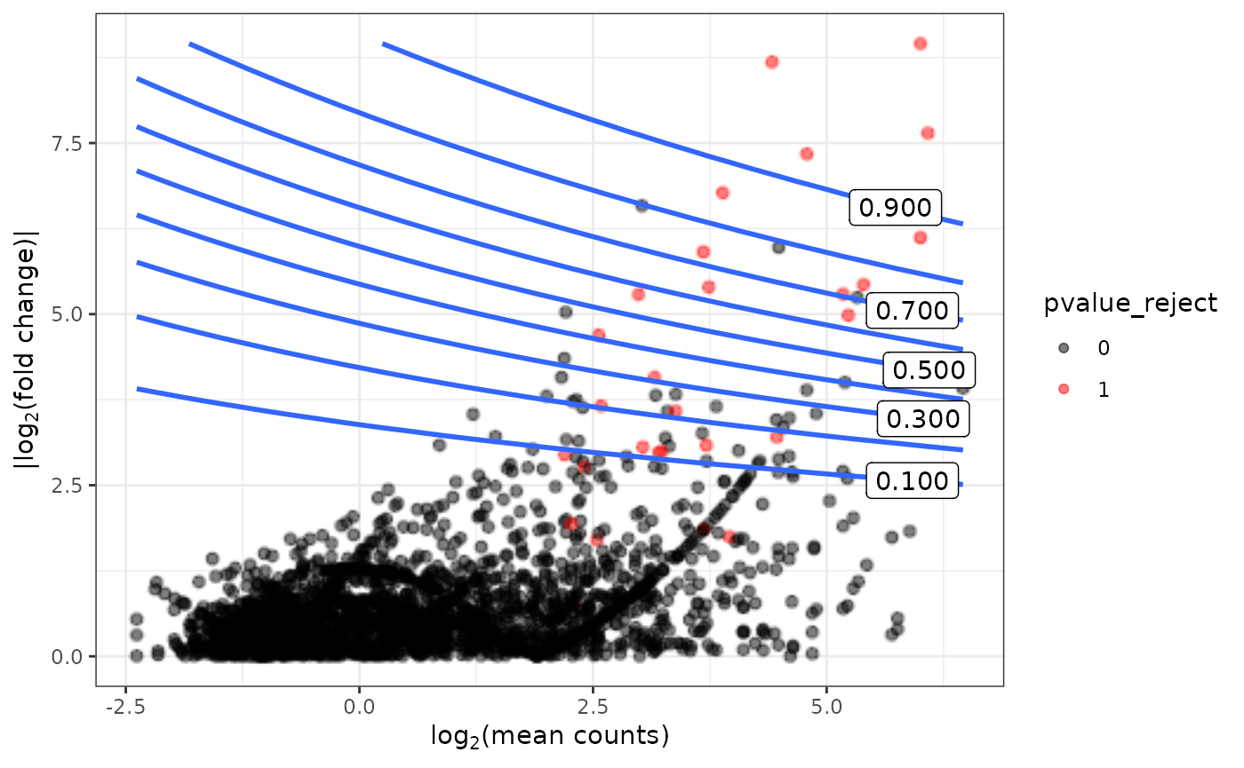
Sample size calculation
Simulate count data for various sample sizes
nsim = 4
nsample_vec = seq(10, 100, 20)
countdata_sims_list  =  list()
for(j in 1:length(nsample_vec)){
  countdata_sims_list[[j]]  =  countdata_sim_fun(logmean_param,
                                                 logfoldchange_param,
                                                 dispersion_param,
                                                 nsamp_per_group = nsample_vec[j],
                                                 ncont  = NULL,
                                                 ntreat = NULL,
                                                 notu,
                                                 nsim = nsim,
                                                 disp_scale = 0.3,
                                                 max_lfc = 15,
                                                 maxlfc_iter = 1000,
                                                 seed = 121)
}

names(countdata_sims_list) = paste0("sample_",nsample_vec)
Estimate p-values associated to fold changes for each taxa for simulated data per sample size
desq_est_list  =  list()
for(i in 1:length(countdata_sims_list)){

  countdata_list       =   countdata_sims_list[[i]]$countdata_list
  metadata_list        =   countdata_sims_list[[i]]$metadata_list
  desq_est_list[[i]]   =   deseq_fun_est(metadata_list =  metadata_list,
                               countdata_list =  countdata_list,
                               alpha_level    =  0.1,
                               group_colname  = "Groups",
                               sample_colname = "Samples",
                               num_cores      =  1,
                               ref_name       = "control")

}
names(desq_est_list) = paste0("sample_",nsample_vec)
Fit Generalized Additive Model (GAM) for power estimation
We now fit a GAM model to predict statistical power. This time, we predict GAM with covariates as mean count of taxa, fold change of taxa and group sample size. Let for denote the sample size per group corresponding to the dataset. For a given dataset, we assume equal sample sizes across all groups. The value of is constant within each dataset but varies across datasets. The GAM model is defined by
where the functions and are two-dimensional smoothing surfaces with basis generated by the tensor product smooth of pairs of and . and are constrained to be monotonically increasing functions.
pow_ss <- readRDS(file.path(extdata_path, "gam_fit_MultiSamples.rds"))
## The code below was used to generate the precomputed
## `gam_fit_MultiSamples.rds` object.
## The saved result is loaded throughout
## this vignette to reduce vignette build times.
# deseq_list = lapply(desq_est_list, function(x){
# read_data(x, "deseq_estimate")
# })
#
# pval_est_list <- lapply(deseq_list, function(sample_list) {
# lapply(sample_list, function(sim_df) {
# sim_df$padj
# })
# })
#
#
# logfoldchange_list = read_data(countdata_sims_list,"logfoldchange_list")
# logmean_list = read_data(countdata_sims_list,"logmean_list")
#
# pow_ss <- power_fun_ss(pval_est_list,
# logmean_list,
# nsample_vec = nsample_vec,
# logfoldchange_list,
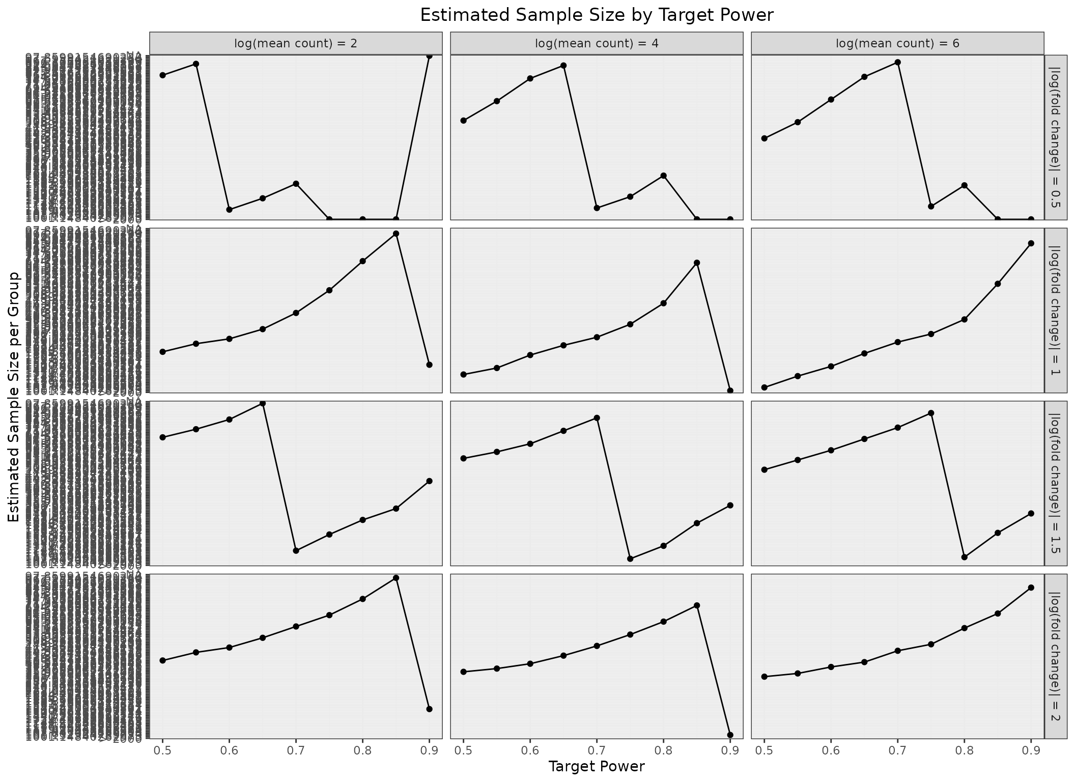
# alpha_level=0.1)Estimate sample size for a given statistical power, fold change and mean abundance
For a given target power, the sample size required to detect a taxon with a given fold change and mean abundance is obtained by a root-finding technique. Let denote the estimated linear predictor from the fitted GAM. The predicted power is obtained via the logistic transformation
Given and a target power , the required sample size is estimated by finding the root of the equation:
target_power =  0.8; model  =  pow_ss$gam_mod; abs_lfc = 1.2; logmean = 4

ss_estimate = uniroot_ss(target_power, logmean, abs_lfc, model,
                        xmin = log2(10), xmax = log2(5000),
                        maxiter = 10000,
                        max_report = 2000)

ss_estimate
## $sample_size_per_group
## [1] 277.471
##
## $conclusion
## [1] "Success."
##
## $predicted_power_min_n
## [1] 0.004765494
##
## $predicted_power_max_n
## [1] 0.9882709
target_power_vec <- seq(0.5, 0.9, 0.05) #c(0.6, 0.7, 0.8, 0.9)
abs_lfc_vec      <- c(0.5, 1.0, 1.5, 2.0)
logmean_vec      <- c(2, 4, 6)

param_grid <- expand.grid(
  target_power = target_power_vec,
  abs_lfc = abs_lfc_vec,
  logmean = logmean_vec
)

param_grid$sample_size_per_group <- apply(
  param_grid,
  1,
  function(x) {
      uniroot_ss(
        target_power = as.numeric(x["target_power"]),
        logmean      = as.numeric(x["logmean"]),
        abs_lfc      = as.numeric(x["abs_lfc"]),
        model        = pow_ss$gam_mod,
        xmin         = log2(10),
        xmax         = log2(5000),
        maxiter      = 10000,
        max_report   = 2000)$sample_size_per_group
  }
)

head(param_grid)
## target_power abs_lfc logmean sample_size_per_group
## 1 0.50 0.5 2 761.879630397996
## 2 0.55 0.5 2 921.650526518332
## 3 0.60 0.5 2 1119.33443287526
## 4 0.65 0.5 2 1370.72189298116
## 5 0.70 0.5 2 1702.19099725221
## 6 0.75 0.5 2 > 2000
ggplot(param_grid,
       aes(x = target_power,
           y = sample_size_per_group,
           group = 1)) +
  geom_line() +
  geom_point() +
  facet_grid(
    abs_lfc ~ logmean,
    labeller = labeller(
      abs_lfc = function(x) paste0("|log(fold change)| = ", x),
      logmean = function(x) paste0("log(mean count) = ", x)
    )
  ) +
    labs(
    x = "Target Power",
    y = "Estimated Sample Size per Group",
    title = "Estimated Sample Size by Target Power"
  ) +
  theme_bw() +
  theme(
    plot.title = element_text(hjust = 0.5)
  )
Appendix
Data description and parameter estimates from actual microbiome datasets
| Dataset <- c(“ArcticFireSoils”, “Blueberry”, “cdi_schubert”, | ||||||||||||
|---|---|---|---|---|---|---|---|---|---|---|---|---|
| ArcticFireSoils | 4 | (0.10,0.38,0.37,0.15) | (-2.81,-1.56,0.31,3.27) | (0.45,0.80,1.35,2.39) | 2 | (-3.88) | ||||||
| Blueberry | 4 | (0.37,0.22,0.29,0.12) | (-0.47,-1.45,0.83,2.54) | (0.71,0.52,1.05,1.66) | 2 | (4.97) | ||||||
| cdi_schubert | 3 | (0.54,0.37,0.09) | (-2.02,0.78,4.17) | (0.94,1.57,2.04) | 2 | (-1.16) | ||||||
| cdi_vincent | 2 | (0.56,0.44) | (3.06,-0.03) | (2.10,0.89) | 2 | (4.93) | ||||||
| Chemerin | 3 | (0.56,0.02,0.42) | (-0.86,0.74,2.27) | (1.14,0.09,2.32) | 2 | (4.52) | ||||||
| crc_baxter | 4 | (0.16,0.33,0.20,0.32) | (-3.13,-2.01,-0.49,2.73) | (0.55,0.76,2.46,1.21) | 2 | (4.65) | ||||||
| crc_zeller | 5 | (0.13,0.40,0.30,0.13,0.03) | (-2.32,-1.33,0.15,2.33,5.75) | (0.50,0.71,1.09,1.70,2.52) | 2 | (3.66) | ||||||
| edd_singh | 1 | 1 | (-0.42) | (2.39) | 2 | (-1.99) | ||||||
| Exercise | 3 | (0.15,0.48,0.36) | (-1.20,0.17,2.39) | (0.50,1.10,1.97) | 2 | (-4.83) | ||||||
| glass_plastic_oberbeckmann | 3 | (0.44,0.50,0.06) | (-0.08,1.91,5.71) | (0.64,1.23,1.18) | 2 | (-3.83) | ||||||
| GWMC_ASIA_NA | 4 | (0.10,0.35,0.38,0.17) | (-4.72,-3.18,-1.17,1.41) | (0.61,0.98,1.50,2.28) | 2 | (4.08) | ||||||
| GWMC_HOT_COLD | 5 | (0.14,0.35,0.37,0.00,0.14) | (-4.73,-3.16,-1.06,-0.93,1.57) | (0.69,1.55,1.05,0.07,2.28) | 2 | (3.58) | ||||||
| hiv_dinh | 3 | (0.49,0.45,0.06) | (0.42,2.15,5.79) | (0.84,1.25,0.70) | 2 | (-2.29) | ||||||
| hiv_lozupone | 3 | (0.30,0.28,0.42) | (-0.12,1.30,3.80) | (0.92,0.50,1.83) | 2 | (-4.86) | ||||||
| hiv_noguerajulian | 4 | (0.09,0.46,0.25,0.19) | (-2.83,-1.71,0.21,3.64) | (0.46,0.75,1.33,2.32) | 2 | (-2.44) | ||||||
| ibd_papa | 3 | (0.06,0.49,0.45) | (0.14,1.71,4.69) | (0.69,0.57,0.98) | 2 | (-1.31) | ||||||
| Ji_WTP_DS | 3 | (0.33,0.30,0.37) | (-0.68,2.61,6.67) | (0.84,2.69,1.84) | 2 | (4.44) | ||||||
| MALL | 3 | (0.39,0.11,0.50) | (-0.65,0.65,3.26) | (0.82,0.40,1.83) | 2 | (4.26) | ||||||
| ob_goodrich | 4 | (0.15,0.16,0.62,0.06) | (-3.89,-2.39,-0.17,3.31) | (0.58,1.61,0.98,2.47) | 2 | (4.90) | ||||||
| ob_ross | 2 | (0.34,0.66) | (-0.58,2.34) | (0.75,1.98) | 2 | (4.40) | ||||||
| ob_turnbaugh | 3 | (0.55,0.03,0.42) | (-0.98,0.14,1.22) | (0.79,0.08,1.66) | 2 | (1.60) | ||||||
| ob_zhu | 3 | (0.57,0.01,0.42) | (-0.12,0.53,2.77) | (0.82,0.04,1.97) | 2 | (-2.12) | ||||||
| ob_zupancic | 3 | (0.45,0.32,0.23) | (-1.98,-0.56,1.91) | (0.87,1.42,0.41) | 2 | (-1.90) | ||||||
| par_scheperjans | 3 | (0.39,0.32,0.28) | (-1.71,-0.31,1.34) | (0.71,1.02,1.58) | 2 | (4.16) | ||||||
| sed_plastic_hoellein | 3 | (0.41,0.39,0.20) | (-0.03,1.46,3.32) | (0.65,1.05,1.67) | 2 | (-4.73) | ||||||
| sed_plastic_rosato | 3 | (0.40,0.43,0.17) | (-0.25,1.58,4.06) | (0.70,1.23,1.93) | 2 | (4.65) | ||||||
| sw_plastic_frere | 5 | (0.06,0.25,0.33,0.27,0.08) | (-1.88,-1.04,0.19,1.93,4.08) | (0.33,0.52,0.83,1.35,2.21) | 2 | (2.68) | ||||||
| t1d_alkanani | 5 | (0.06,0.30,0.47,0.15,0.02) | (-3.06,-2.54,-1.91,-0.87,0.82) | (0.17,0.30,0.46,0.72,1.37) | 5 | (0.23,-2.85,-4.30,4.83) | ||||||
| t1d_mejialeon | 2 | (0.47,0.53) | (0.73,3.57) | (0.92,1.94) | 2 | (-2.93) | ||||||
| wood_plastic_kesy | 3 | (0.29,0.42,0.29) | (-1.16,1.16,4.65) | (0.70,1.43,2.46) | 2 | (3.96) |
Acknowledgments
We would like to express our sincere gratitude to Dr. Jacob T. Nearing for his generosity in granting us access to the 38 microbiome datasets used in the paper “Microbiome differential abundance methods produce different results across 38 datasets” (Nearing et al. 2022). These datasets were invaluable in developing, testing, and validating this R package for power and sample size calculation in microbiome studies.
We also sincerely appreciate the following individuals for running the functions in this package on the microbiome datasets published in (Nearing et al. 2022), thereby providing users with plausible parameter values for their research work: Alim Tuguzbay, Arjya Bhattacharjee, Atiyah Sulaiman, George Vinichenko, Josh Effero, Mahdiya Adnan, Mir Akbaar Khaled, Nevin Xu, Nicole Padoun, Riya Srivastava, and Shaira Habib (University of Alberta: Alim Tuguzbay, Arjya Bhattacharjee, Atiyah Sulaiman, George Vinichenko, Josh Effero, Mahdiya Adnan, Mir Akbaar Khaled, Nevin Xu, and Shaira Habib; McMaster University: Nicole Padoun and Riya Srivastava.